summary

I was learning about Stein estimation from a friend of mine, and when I was studying machine learning, I saw the term “Stein estimator” written somewhere in a paper, so I decided to study estimators. I still do not understand the proof of why the Stein estimator reduces the error, so I will continue to study it,

What is Stein Presumption?

It is one of the methods that can provide more accurate estimates than the least squares method when many population means are estimated simultaneously. It is a kind of so-called reduced estimator. Suppose that there are $N$ mothers $x_1$ , $x_2$ , $x_3$ , , , $x_N$ and that for each $x_i$ we observe independent random variables $z_1$ , $z_2$ , , , $z_N$ that follow a normal distribution $N(x_i,\sigma)$ with variance $\sigma$ . The natural estimator of $x_i$ is $z_i$ itself, and $z_i$ is a minimum variance unbiased estimator and a maximum likelihood estimator. When trying to estimate $x_i$ based on $z_i$ , we basically base it on the mean squared error $(MSE)$ . At this time, whatever the value of $x_i$ is, it is said that there is no estimator that is smaller than the sum of the MSEs.
$\sum_{i=1}^{N} E{(\hat{x_i}-x_i)^2}$

However, when $N$ is greater than 3, there exists an estimator such that the sum of the MSEs is smaller. That is the James-Stein estimator. However, when $N=1,2$ , z is admissible, and for $N\geq3$ , z is non-admissible and is improved by the James-Stein estimator.
$\delta = (1-\frac{N-2}{||Z||^2})*z_i$

※ $||Z||^2$ denotes the Euclidean norm. Furthermore, the Stein estimator, which can be better estimated than the James-Stein estimator, consists of the following equation.

$\delta = (1-a)z_i+\frac{N}{a} \sum_{i=1}^{N} y_i$
$a = \frac{\sigma^2}{s^2}$
$s^2 = \frac{1}{N-3} \sum_{i=1}^{N} (y_i - \frac{1}{N}\sum_{i=1}^{n} y_i)^2$

Validation (James-Stein estimator and MSE)

The following R program creates samples that follow a normal distribution $N(x_i,\sigma)$ with variance $\sigma=1$ for each $x_i$ for 10 populations $x_i$ , $x_2$ , , , $x_{10}$ (1,2,3, , ,10) respectively. To compare the estimation, the sum of the MSE and James-Stein estimator for each sample is the expected value of the squared error

$E[\sum_{i=1}^{N} (({z_i}-x_i)^2)]$

$E[\sum_{i=1}^{N} (({\delta_i}-x_i)^2)]$

I would like to compare the estimates with the difference in

n <- 10 mu <- 1:n sig <- 1 try_num = 1000 mat <- matrix(0, 1, 2) ## n個のサンプルを発生させる 
tmp <- rnorm(n, mu, sig) xx<-norm(tmp, type="2")^2 ## James-Stein推定値を求める 
Stein <- (1-(n-2)/(xx)) * tmp ## 結果を保存 
mat[1, 1] <- sum((Stein - mu)^2)/n # James-Stein推定値を用いた二乗誤差の期待値 
mat[1, 2] <- sum((tmp - mu)^2)/n # データそのものを用いた二乗誤差の期待値 
paste("James-Stein : ", mean(mat[, 1])) paste("MSE : ", mean(mat[, 2]))

We found that the James-Stein estimation had a smaller squared error by doing the following number of times.

> paste("James-Stein : ", mean(mat[, 1])) [1] "James-Stein : 0.566820964708058" > paste("MSE : ", mean(mat[, 2])) [1] "MSE : 0.598717547433325"
> paste("James-Stein : ", mean(mat[, 1])) [1] "James-Stein : 0.697318338422813" > paste("MSE : ", mean(mat[, 2])) [1] "MSE : 0.680173749274679"

Next we will try 1000 attempts.

n <- 10 mu <- 1:n sig <- 1 try_num = 1000 mat <- matrix(0, try_num, 2) ## 1000回実行します 
for(i in 1:try_num){ ## サンプルを発生させる
  tmp <- rnorm(n, mu, sig) 
  xx<-norm(tmp, type="2")^2 ## スタイン推定値を求める 
  Stein <- (1-(n-2)/(xx)) * tmp ## 結果を保存する 
  mat[i, 1] <- sum((Stein - mu)^2)/n # スタイン推定値を用いた二乗誤差の期待値 
  mat[i, 2] <- sum((tmp - mu)^2)/n # データそのものを用いた二乗誤差の期待値
} 
paste("Stein : ", mean(mat[, 1])) paste("MSE : ", mean(mat[, 2]))

As a result, the Stein estimate has a smaller expected value of squared error than the James-Stein estimate.

> paste("Stein : ", mean(mat[, 1])) [1] "Stein : 0.980164575967686" > paste("MSE : ", mean(mat[, 2])) [1] "MSE : 0.994713532652209"

Verification (when N increases)

I would like to visualize how each estimate changes when the $N$ number of matrices $x_1$ , $x_2$ , $x_3$ , , , $x_N$ increases from 1,2,3…. I would like to visualize how each estimate changes as $x_N$ increases from 1,2,3….

MSE<-c(0,0,0,0,0,0,0,0,0,0,0,0,0,0,0,0,0,0,0,0,0,0,0,0,0,0,0,0,0,0)
j_s<-c(0,0,0,0,0,0,0,0,0,0,0,0,0,0,0,0,0,0,0,0,0,0,0,0,0,0,0,0,0,0)
s<-c(0,0,0,0,0,0,0,0,0,0,0,0,0,0,0,0,0,0,0,0,0,0,0,0,0,0,0,0,0,0)

S1<-0
S2<-0
S3<-0

n   <- 30
sig <- 1

try_num = 1000
mat <- matrix(0, try_num, 3)

for(j in 1:n){
    mu  <- 1:j

    for(i in 1:try_num){
        ## サンプルを発生させる
        tmp <- rnorm(j, mu, sig)
        xx<-norm(tmp, type="2")^2

        ## James-stein推定値を求める
        if(j>2){
            j_stein  <- (1-(j-2)/(xx)) * tmp  
        }else{
            j_stein  <- (1-(1)/(xx)) * tmp 
        }   

        ## stein推定値を求める
        if(j>3){
            s_2 <- (1/(j-3)) * sum((tmp - mean(tmp))^2) 
            a   <- (sig)^2 / s_2
            stein <- (1-a)*tmp + (a/j)*sum(tmp)
        }else{
            s_2 <- sum((tmp - mean(tmp))^2) 
            a   <- (sig)^2 / s_2
            stein <- (1-a)*tmp + (a/j)*sum(tmp)
        }

        ## 結果を保存する
        S1 <- S1 + sum((tmp - mu)^2)/j # データそのものを用いた二乗誤差の期待値
        S2 <- S2 + sum((j_stein - mu)^2)/j # スタイン推定値を用いた二乗誤差の期待値
        S3 <- S3 + sum((stein - mu)^2)/j # データそのものを用いた二条誤差の期待値
    }
    MSE[j] <- S1/100
    j_s[j] <- S2/100
    s[j]   <- S3/100

    S1<-0
    S2<-0
    S3<-0
}

print(MSE)
print(j_s)
print(s)

z<-1:30

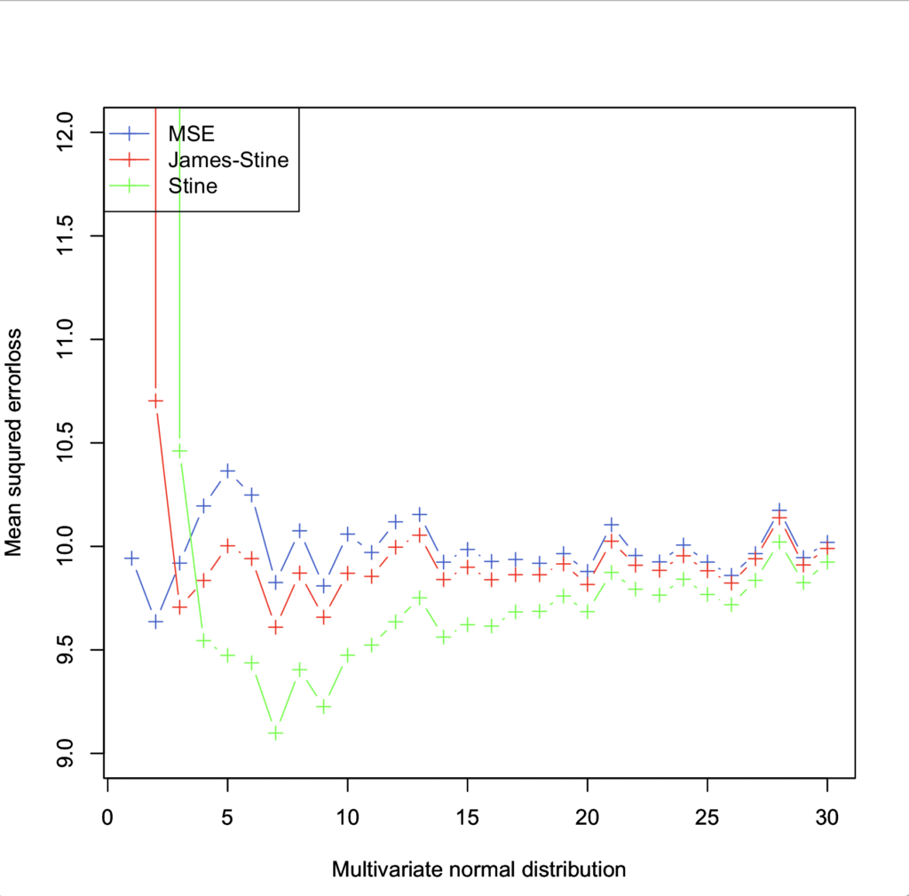
plot(z,MSE,xlab="Multivariate normal distribution",ylab="Mean suqured errorloss",pch=3,ylim=c(9,12),type="b",col="royalblue3")
par(new=T)
plot(z,j_s,xlab="Multivariate normal distribution",ylab="Mean suqured errorloss",pch=3,ylim=c(9,12),type="b",col="red")
par(new=T)
plot(z,s,xlab="Multivariate normal distribution",ylab="Mean suqured errorloss",pch=3,ylim=c(9,12),type="b",col="green")

legend("topleft",
    legend=c("MSE", "James-stein", "stein"),
    pch=c(3,3,3),
    lty=c(1,1,1),
    col=c("royalblue3", "red", "green")
    )

The results show that Stein estimation < James_Stein estimation < MSE and the squared error is less, indicating that Stein estimation is a better estimation.

> print(MSE)
 [1]  9.893811 10.061190 10.201689  9.991315 10.099179  9.872469  9.984524 10.109032 10.170069  9.929639 10.090521 10.132484 10.112773
[14]  9.938398  9.938122 10.129706 10.003247  9.966152  9.884785  9.984538  9.998484  9.988337  9.895186  9.989390  9.991495 10.203533
[27] 10.052179  9.987638  9.908004 10.070632
> print(j_s)
 [1] 1670.078472   11.068689    9.930817    9.705076    9.762386    9.590761    9.726514    9.909983    9.943457    9.762370
[11]    9.961938   10.015718    9.997933    9.850449    9.864478   10.045977    9.931580    9.881776    9.816021    9.915127
[21]    9.959294    9.935525    9.850859    9.950460    9.958395   10.168994   10.009156    9.950454    9.874517   10.045453
> print(s)
 [1]          NaN 1.399345e+06 1.174287e+01 1.004977e+01 9.381920e+00 9.156616e+00 9.240040e+00 9.404127e+00 9.449622e+00 9.308097e+00
[11] 9.572499e+00 9.637781e+00 9.720924e+00 9.597115e+00 9.675648e+00 9.830977e+00 9.691651e+00 9.719077e+00 9.626047e+00 9.749151e+00
[21] 9.801033e+00 9.801899e+00 9.749940e+00 9.828186e+00 9.872554e+00 1.003455e+01 9.914897e+00 9.867066e+00 9.815286e+00 9.956238e+00
>

About Stein Presumption

summary

What is Stein Presumption?

Validation (James-Stein estimator and MSE)

Verification (when N increases)

summary

Leave a Comment Cancel